Trig composition table

I’ve written a couple posts that reference the table below.

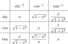
$\renewcommand{\arraystretch}{2.2} \begin{array}{c|c|c|c} & \sin^{-1} & \cos^{-1} & \tan^{-1} \\ \hline \sin & x & \sqrt{1-x^{2}} & \dfrac{x}{\sqrt{1+x^2}} \\ \hline \cos & \sqrt{1-x^{2}} & x & \dfrac{1}{\sqrt{1 + x^2}} \\ \hline \tan & \dfrac{x}{\sqrt{1-x^{2}}} & \dfrac{\sqrt{1-x^{2}}}{x} & x \\ \end{array}$

You could make a larger table, 6 × 6, by including sec, csc, cot, and their inverses, as Baker did in his article [1].

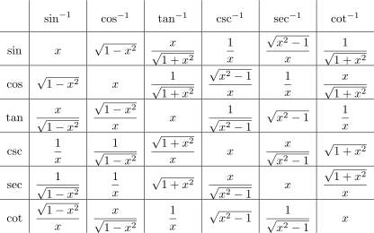
Note that rows 4, 5, and 6 are the reciprocals of rows 1, 2, and 3.

Returning to the theme of the previous post, how could we verify that the expressions in the table are correct? Each expression is one of 14 forms for reasons we’ll explain shortly. To prove that the expression in each cell is the correct one, it is sufficient to check equality at just one random point.

Every identity can be proved by referring to a right triangle with one side of length x, one side of length 1, and the remaining side of whatever length Pythagoras dictates, just as in the first post [2]. Define the sets A, B, and C by

A = {1}
B = {x}
C = {√(1 − x²), √(x² − 1), √(1 + x²)}

Every expression is the ratio of an element from one of these sets and an element of another of these sets. You can check that this can be done 14 ways.

Some of the 14 functions are defined for |x| ≤ 1, some for |x| ≥, and some for all x. This is because sin and cos has range [−1, 1], sec and csc have range (−∞, 1] ∪ [1, ∞) and tan and cot have range (−∞, ∞). No two of the 14 functions are defined and have the same value at more than a point or two.

The follow code verifies the identities at a random point. Note that we had to define a few functions that are not built into Python’s math module.

    from math import *

    def compare(x, y):
        print(abs(x - y) < 1e-12)

    sec  = lambda x: 1/cos(x)    
    csc  = lambda x: 1/sin(x)
    cot  = lambda x: 1/tan(x)
    asec = lambda x: atan(sqrt(x**2 - 1))
    acsc = lambda x: atan(1/sqrt(x**2 - 1))
    acot = lambda x: pi/2 - atan(x)

    x = np.random.random()
    compare(sin(acos(x)), sqrt(1 - x**2))
    compare(sin(atan(x)), x/sqrt(1 + x**2))
    compare(sin(acot(x)), 1/sqrt(x**2 + 1))
    compare(cos(asin(x)), sqrt(1 - x**2))
    compare(cos(atan(x)), 1/sqrt(1 + x**2))
    compare(cos(acot(x)), x/sqrt(1 + x**2))
    compare(tan(asin(x)), x/sqrt(1 - x**2))
    compare(tan(acos(x)), sqrt(1 - x**2)/x)
    compare(tan(acot(x)), 1/x)
    
    x = 1/np.random.random()
    compare(sin(asec(x)), sqrt(x**2 - 1)/x)
    compare(cos(acsc(x)), sqrt(x**2 - 1)/x)    
    compare(sin(acsc(x)), 1/x)
    compare(cos(asec(x)), 1/x)
    compare(tan(acsc(x)), 1/sqrt(x**2 - 1))
    compare(tan(asec(x)), sqrt(x**2 - 1))

This verifies the first three rows; the last three rows are reciprocals of the first three rows.

[1] G. A. Baker. Multiplication Tables for Trigonometric Operators. The American Mathematical Monthly, Vol. 64, No. 7 (Aug. – Sep., 1957), pp. 502–503.

[2] These geometric proofs only prove identities for real-valued inputs and outputs and only over limited ranges, and yet they can be bootstrapped to prove much more. If two holomorphic functions are equal on a set of points with a limit point, such as a interval of the real line, then they are equal over their entire domains. So the geometrically proven identities extend to the complex plane.

The post Trig composition table first appeared on John D. Cook.

Trig composition table

AI 摘要

Related posts